How Search Works in Production: From Inverted Indexes to Tail Latency

Search looks deceptively simple from the outside.

A user sends:

"best noise cancelling headphones"

and a few milliseconds later gets a ranked list of useful results.

The implementation behind that response is rarely “run one search algorithm.”

Production search is usually a multi-stage retrieval and ranking system. It starts by finding a relatively large set of plausible candidates, progressively spends more computation deciding which candidates are actually relevant, and finally tries to do all of that within a latency budget while indexes are changing underneath it.

A useful mental model is:

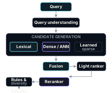
The interesting engineering problems start when the corpus becomes large, the index must stay fresh, queries fan out across machines, and “average latency” stops being a useful number.

This article walks through that system from the bottom up.

---

1. The Foundation: The Inverted Index

For lexical search, the core data structure is still the inverted index.

Instead of storing:

document -> terms

for retrieval, we build:

term -> documents containing that term

Conceptually:

"android" -> [doc 2, doc 8, doc 15, doc 21]
"search"  -> [doc 1, doc 8, doc 17]
"kotlin"  -> [doc 2, doc 5, doc 21]

Those document lists are called posting lists.

Real implementations store more than document IDs. Depending on the field and query features, postings can also include term frequency, positions, offsets, and payload information.

How Lucene stores this efficiently

Lucene, the engine underneath Elasticsearch, OpenSearch, and Solr, does considerably more than keep a giant hash map in memory.

Modern Lucene codecs organize terms into blocks based on shared prefixes. A compact term index helps locate the relevant block quickly, while the actual term dictionary and postings remain stored in index files. This is more precise than saying “the entire term dictionary is an FST.”

Posting lists are compressed because document IDs are monotonically increasing. Instead of storing:

[1001, 1007, 1010, 1030]

we can encode deltas:

[1001, 6, 3, 20]

Modern Lucene postings formats then encode large runs using packed integer blocks, with variable-length encoding for smaller tails. This reduces both storage and memory bandwidth.

Lucene also stores doc values, a column-oriented representation used for operations such as sorting, faceting, and aggregations.

This gives us two different access patterns:

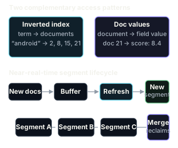
Both are important in production search.

---

2. Segments: Why Search Indexes Are Nearly Immutable

A Lucene index is not one giant mutable data structure.

It is composed of segments.

Each segment is effectively an immutable mini-index. Newly indexed documents accumulate and eventually become new segments. Existing segments are not rewritten every time a document changes.

Deletes are initially represented logically rather than immediately rewriting every affected file. Segment merges later combine segments and reclaim deleted data.

This architecture is one of the reasons Lucene can support high read concurrency efficiently.

It also creates an important operational tradeoff.

More frequent indexing creates more small segments. More segments increase search overhead and eventually create merge work. Merges consume CPU, disk bandwidth, and filesystem cache bandwidth, the same resources your searches want.

Refresh is not the same as durability

A refresh makes newly indexed documents searchable.

A durable Lucene commit/Elasticsearch flush is a different operation.

In current Elasticsearch, background refreshes normally happen every second for indices receiving search traffic; idle indices can skip those periodic refreshes. Elastic Serverless currently uses a five-second default.

That creates a straightforward tradeoff:

shorter refresh interval
        ↓
fresher search results
        ↓
more refresh/segment overhead

For a search-heavy application where one-second freshness is unnecessary, increasing the refresh interval can materially improve indexing throughput.

Search freshness is therefore not free. It is part of your system’s resource budget.

---

3. BM25: Still an Extremely Strong Baseline

Once we have candidate documents, we need to score them.

Lucene’s default lexical similarity is BM25.

A simplified form is:

score(D, Q) =
    Σ IDF(t) *
      f(t,D) * (k1 + 1)
      ------------------------------
      f(t,D) + k1 * (1 - b + b * |D| / avgdl)

The important ideas matter more than memorizing the equation.

Term frequency saturation: mentioning a query term twice is useful; mentioning it for the 500th time should not make a document 500 times more relevant.

Inverse document frequency: rare terms carry more information than terms appearing almost everywhere.

Document-length normalization: longer documents naturally contain more term occurrences, so raw frequency needs normalization.

Lucene currently defaults to k1 = 1.2 and b = 0.75.

BM25 remains difficult to beat for queries containing exact identifiers, product codes, names, technical terminology, rare phrases, and other cases where exact token overlap contains valuable information.

This is why “we added embeddings, therefore BM25 is obsolete” is usually the wrong conclusion.

BEIR’s cross-domain evaluation famously found BM25 to be a robust zero-shot baseline, while more sophisticated reranking and late-interaction systems generally achieved higher effectiveness at greater computational cost.

A distributed-search subtlety: BM25 statistics are not always global

Once the index is sharded, another complication appears.

Each shard is itself a Lucene index and therefore has its own term statistics.

Elasticsearch’s default query_then_fetch mode scores using shard-local term and document frequencies. Usually, with enough evenly distributed data, the statistics are similar enough that this works well.

For cases where shard-level differences materially affect ranking, dfs_query_then_fetch first collects global term statistics, but adds another distributed round trip.

So even a seemingly pure relevance question can become a distributed-systems tradeoff.

---

4. How Search Avoids Scoring Everything

An inverted index tells us which documents contain a query term.

That does not mean a production engine blindly scores every matching document.

For common terms, a posting list may contain millions of documents. Exhaustively scoring them all would waste enormous amounts of CPU.

Search engines therefore use dynamic pruning.

Algorithms such as MaxScore, WAND, and Block-Max WAND maintain upper bounds on how much score a document or block could still contribute.

If a candidate cannot possibly beat the current top-k threshold, the engine can skip it.

Conceptually:

Current kth-best score = 12.4

Maximum score this postings block could achieve = 7.8

7.8 < 12.4
→ skip the block

This is a major reason lexical retrieval remains extraordinarily efficient.

The same principle appears repeatedly throughout production search:

Do expensive work only on candidates that still have a realistic chance of winning.

That principle will show up again in ANN retrieval, multi-stage ranking, and reranking.

---

5. Semantic Search: Dense Retrieval

BM25 understands words.

Dense retrieval attempts to represent meaning.

A bi-encoder independently converts the query and each document into vectors:

query    -> encoder -> [0.17, -0.32, ...]
document -> encoder -> [0.14, -0.29, ...]

Documents can be embedded ahead of time. At query time we only embed the query and find nearby document vectors.

Similarity is commonly measured using cosine similarity, dot product, or Euclidean distance.

The problem is scale.

For one million 768-dimensional float32 embeddings, brute-force comparison means touching roughly:

1,000,000 × 768

dimensions for every query.

At larger scales, exact scanning quickly becomes too expensive.

That leads to Approximate Nearest Neighbor search, or ANN.

---

6. ANN: Trading Perfect Recall for Speed

ANN indexes deliberately avoid examining every vector.

The goal is not:

Find the mathematically exact nearest neighbors at any cost.

The production goal is closer to:

Find almost all of the useful nearest neighbors while meeting the latency and resource budget.

Three common approaches are HNSW, IVF/PQ, and disk-oriented graph indexes such as DiskANN.

Approach	Basic idea	Main advantage	Main tradeoff
HNSW	Navigate a multi-layer proximity graph	Excellent recall/latency	Memory-heavy working set
IVF	Partition vectors into clusters and probe selected clusters	Tunable search cost	Recall depends heavily on probing
IVF-PQ	IVF plus compressed vector codes	Very low vector footprint	More approximation error
DiskANN-style graph	Design graph traversal around SSD access	Large indexes with lower RAM requirements	More complex build/serving model

HNSW

HNSW builds a navigable graph of nearby vectors.

Instead of checking every vector, search begins from entry points and repeatedly moves toward promising neighbors.

Its important tuning parameters include:

M

which controls graph connectivity,

efConstruction

which controls effort spent building the graph, and

efSearch

or an implementation-specific equivalent controlling query-time exploration.

Higher search effort generally produces better recall but also higher latency.

That gives us one of the central search-engineering curves:

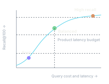
There is no universally correct point on that curve.

A recommendation search, security search, e-commerce search, and autocomplete service may all make different choices.

The memory-working-set problem

HNSW traversal performs many effectively random accesses across the graph and vectors.

That is fast when the hot working set stays in memory.

As the working set increasingly requires storage access, latency can deteriorate sharply.

It is more accurate to call this a memory-working-set cliff than to say HNSW simply “does not work on disk.”

Modern Elasticsearch explicitly recommends sizing HNSW so the required vector working set fits available off-heap memory and offers int8, int4, binary quantization, and disk-oriented alternatives to reduce that footprint.

DiskANN approached the same systems problem from another direction: design the graph and search process around SSD access, keeping compact representations in memory. Its original paper demonstrated billion-vector search on a single machine with high recall and low reported latency on its benchmark configuration. Those results are impressive, but they are measurements, not universal guarantees.

---

7. Learned Sparse Retrieval: Between BM25 and Dense Search

Dense retrieval is not the only way to add semantics.

Models such as SPLADE generate sparse learned term vectors.

Instead of representing a document as a 768-dimensional dense vector, they assign learned weights to vocabulary terms and can introduce expansion terms that were not present literally in the original text.

The useful property is that the representation remains sparse enough to use inverted-index infrastructure.

So we get something like:

document
   │
   ▼
transformer
   │
   ▼
{
  "android": 2.7,
  "mobile": 1.9,
  "kotlin": 2.3,
  "application": 0.8
}

SPLADE was explicitly designed to combine learned semantic representations with the desirable properties of inverted indexes.

The tradeoff is that learned sparse representations often activate more postings than traditional BM25 queries. That can make pruning less effective and retrieval more expensive.

The broader lesson is useful:

Lexical vs. semantic is not actually a binary choice.

There is an entire design space between classical sparse retrieval and dense vectors.

---

8. Hybrid Retrieval: Let Different Retrievers Fail Differently

Lexical and dense retrieval have different failure modes.

Consider:

Query: "iphone 15 pro max A3108"

Exact lexical matching is extremely valuable.

Now consider:

Query: "phone with a really good camera for night photos"

Semantic retrieval becomes more useful.

A production system can run both.

The problem is that their scores are not directly comparable.

A BM25 score of:

17.8

does not have a meaningful mathematical relationship with a cosine similarity of:

0.83

One solution is score normalization.

Another is Reciprocal Rank Fusion (RRF).

RRF ignores raw scores and combines rank positions:

RRF(d) = Σ 1 / (k + rank(d))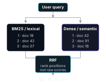

If a document ranks well in several retrieval systems, its fused score increases.

RRF is attractive operationally because it does not require the lexical and vector scoring functions to share a scale. The original RRF work showed that surprisingly simple rank fusion could outperform individual ranking systems.

A rank constant around 60 is common; OpenSearch currently uses 60 as its default.

But hybrid search should not be marketed as magic.

Sometimes BM25 wins. Sometimes dense retrieval wins. Sometimes hybrid wins.

The correct answer is empirical:

BM25
vs
dense
vs
hybrid

on your queries, your relevance labels, and your corpus.

---

9. Retrieval Is Only the First Stage

Candidate generation optimizes primarily for recall.

Suppose the truly relevant document never makes it into the initial 1,000 candidates.

No reranker can rescue it.

This makes the retrieval funnel look something like:

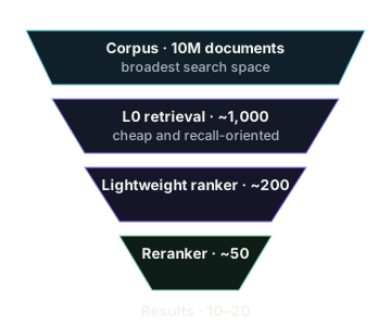
The exact numbers vary enormously by product.

The architecture matters more than the numbers.

Earlier stages are cheap and broad.

Later stages are expensive and selective.

Learning to Rank

Traditional production rankers frequently combine heterogeneous features:

BM25 score
freshness
popularity
click history
document quality
query-document features
personalization
business signals

Gradient-boosted decision trees and LambdaMART-style learning-to-rank models remain strong choices for this type of tabular ranking problem.

Neural models become increasingly attractive when raw text and learned representations carry substantial signal, but their serving cost matters.

This is why multi-stage ranking exists in the first place.

---

10. Cross-Encoders and Late Interaction

Bi-encoders encode query and document separately.

A cross-encoder processes them jointly:

[query + document] -> transformer -> relevance score

That allows much richer interaction between the query and document.

It is also far more expensive because the document representation cannot simply be precomputed and reused in the same way.

Cross-encoders therefore normally rerank a relatively small candidate set rather than the entire corpus.

ColBERT: a middle ground

Late-interaction architectures such as ColBERT independently encode query and document tokens but preserve multiple token-level vectors.

At query time, they compute interactions such as MaxSim between those token representations.

This retains significantly more fine-grained information than a single dense vector while allowing much of the document computation to happen offline.

PLAID later optimized ColBERTv2 retrieval by aggressively pruning low-value candidates using centroid-level interactions; its reported experiments achieved large CPU/GPU speedups while preserving retrieval quality.

Again, the architectural pattern is the important part:

cheap retrieval
      ↓
fewer documents
      ↓
richer interaction
      ↓
better ranking

---

11. Distributed Search: Scatter, Gather, Fetch

Eventually one machine is not enough.

The index is divided into shards.

A typical Elasticsearch search uses query then fetch.

During the query phase, the coordinating node sends the request to one copy of each relevant shard.

Each shard computes its local best candidates and returns lightweight metadata such as document IDs, scores, and sort values.

The coordinator merges those shard-local rankings into the global top-k.

Only then does the fetch phase retrieve the actual source data for the winning documents.

Conceptually:

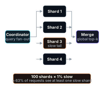
This avoids shipping entire documents for candidates that will never be returned.

It also creates the first major production-search problem.

---

12. Tail Latency: The Slowest Shard Wins

Suppose a query fans out to 100 backends.

If each backend has a 1% probability of entering a slow tail, the chance of the overall request encountering at least one slow backend is:

1 - 0.99^100 ≈ 63%

That is the core observation behind Dean and Barroso’s The Tail at Scale.

Even rare backend stalls become common at the request level when enough machines participate.

The paper reports a Google example where an operation with roughly 10ms single-request p99 grew to around 140ms p99 when waiting for all responses in a 100-way fan-out.

That number comes from the measured distribution, not from the 63% equation alone.

The causes of tail latency are boring individually and brutal collectively:

GC pauses, CPU contention, hot shards, storage stalls, kernel scheduling, noisy neighbors, lock contention, queueing, network variability.

Production systems therefore use techniques such as adaptive replica selection, request hedging, load shedding, micro-partitioning, and selective replication.

The fundamental lesson is:

In a fan-out architecture, you are designing for the maximum latency of many components, not the average latency of one component.

This is why p99 often matters more than mean latency in search.

---

13. Deep Pagination: OFFSET 100000 Does Not Scale Nicely

Distributed ranking makes deep offset pagination expensive.

Imagine:

from = 100000
size = 20

Each shard cannot simply return twenty documents.

It needs enough local candidates for the coordinator to determine which documents belong at global positions 100001–100020.

That creates large per-shard priority queues and substantial wasted work.

Elasticsearch therefore defaults index.max_result_window to 10,000.

For deep, user-facing pagination, search_after avoids repeatedly paying the full offset cost.

If the index is changing while the user pages through results, Point in Time (PIT) + search_after provides a consistent view.

Elasticsearch explicitly recommends this approach for deep pagination. The Scroll API still exists, but is no longer the recommended mechanism for interactive deep pagination; it remains useful for large extraction and reindex-style workflows.

---

14. Index Freshness: The Dual-Write Problem

Search usually is not the source of truth.

Imagine an application writes:

PostgreSQL

and also needs:

Elasticsearch

updated.

The naive implementation is:

write database
write search index

Now crash between those operations.

Congratulations: you have discovered distributed consistency.

A safer architecture commonly uses a transactional outbox or change-data-capture pipeline:

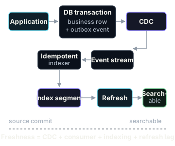
The database write and event creation occur atomically.

The downstream indexing path is normally designed for at-least-once delivery, which means the indexer should be idempotent.

Now search freshness becomes measurable across CDC lag, consumer lag, indexing, and refresh.

That entire duration matters, not merely Elasticsearch’s refresh interval.

---

15. Reindexing Is a Normal Production Operation

Some search changes cannot be applied safely in place.

Changing analyzers, tokenization, field structure, or embedding models often requires rebuilding the index.

A standard migration is:

old index
   │
   ├──────── serves traffic
   │
   ▼
source data
   │
   ▼
new index
   │
   ▼
backfill + validate
   │
   ▼
alias / routing switch

The new index can be built and tested independently before traffic moves.

For embedding-model changes, this is particularly important.

Vectors created by different embedding models, or incompatible versions of the same model, should generally not be mixed in one similarity space unless the model explicitly guarantees compatibility.

A static embedding does not “drift” by itself.

Instead, retrieval quality can degrade because the documents change, the query population changes, the domain changes, or the model changes.

That distinction matters.

---

16. Shards: Parallelism With a Bill Attached

Sharding gives us horizontal scale.

It also gives us:

more network calls
more coordination
more metadata
more merge work
more recovery work
more opportunities for a slow shard

Current Elastic guidance suggests that shards in roughly the 10–50GB range and below around 200 million documents work well for many workloads, but explicitly treats this as guidance rather than a hard rule.

The right shard count depends on query concurrency, document size, ingestion rate, recovery requirements, hardware, routing, and the number of shards each query must touch.

Custom routing can reduce fan-out:

tenant_id -> shard

but introduces another risk.

If one tenant generates 40% of the traffic, congratulations: you have built a hot shard.

Production search is full of tradeoffs like this.

---

17. Memory: Heap Is Only Half the Story

A common mistake with Elasticsearch is to give the JVM as much memory as possible.

Lucene needs the opposite balance.

The JVM needs enough heap for Elasticsearch’s object-heavy runtime structures and caches, but the operating system also needs substantial memory for the filesystem cache.

Elastic currently recommends setting the heap to no more than 50% of available memory and keeping it below the JVM’s compressed ordinary object pointer threshold. That threshold varies by system; Elastic currently describes roughly 26GB as safe on most systems and up to around 30GB on some systems.

So avoid turning:

"keep heap below roughly 30GB"

into:

"31GB is a universal JVM law"

It is not.

Lucene can memory-map index files and relies heavily on the OS filesystem cache for efficient access.

This creates another nonlinear performance boundary.

If the active index fits comfortably in filesystem cache, many reads behave like memory accesses.

Once the working set exceeds available memory, page faults and storage IO become increasingly visible in query latency.

Search sizing is therefore often about the hot working set, not just total index bytes.

---

18. Caching: Search Gives You Several Ways to Be Confused

Search traffic is often heavy-tailed: some queries repeat frequently while a long tail appears only occasionally.

That makes caching valuable.

But “the search cache” is not one cache.

In Elasticsearch, the node query cache can cache eligible filter-context query results on a per-segment basis using reuse heuristics.

The shard request cache caches shard-level responses. By default, it mainly benefits size=0 searches such as aggregation-heavy requests, and entries are invalidated when a shard refreshes.

Below both sits the filesystem page cache.

Applications may add another result cache.

A CDN may cache head queries again.

Cache invalidation remains cache invalidation; search just gives you enough cache layers to make it a team sport.

For very hot queries, another concern is the cache stampede: one entry expires and hundreds of requests simultaneously attempt the same expensive recomputation.

Request coalescing, staggered expiration, and controlled stale serving can help.

---

19. Recall vs. Latency Is the Central Runtime Tradeoff

Search quality is not independent of serving cost.

Almost every retrieval stage exposes some version of the same control.

Decision	More expensive setting usually gives	Cost
HNSW exploration	Higher ANN recall	More CPU / memory accesses / latency
IVF probes	Higher ANN recall	More candidate comparisons
Retrieval depth	More candidates reach ranking	More ranking work
Rerank depth	Better final ranking opportunity	More model inference
Higher-precision vectors	Less quantization error	More RAM / bandwidth
More shards queried	Greater corpus coverage	More fan-out / tail risk

This is why production search teams should plot quality against latency, not report them independently.

For ANN, for example:

ef / candidate exploration
      ↓
Recall@100
      ↓
p50 / p95 / p99 latency

The question is not:

Which setting produces the highest recall?

It is:

Where is the best quality point that still satisfies the latency and cost budget?

---

20. Graceful Degradation

Suppose your normal pipeline is:

BM25 + ANN
    ↓
hybrid fusion
    ↓
ML ranker
    ↓
cross-encoder
    ↓
results

Under overload, returning nothing after three seconds may be worse than returning a slightly weaker ranking in 150ms.

A search service can therefore degrade intentionally:

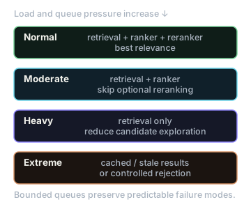
ANN exploration can sometimes be reduced.

Reranking depth can be reduced.

Optional features can be disabled.

Requests may be rejected before queues become unbounded.

The key word is intentional.

Random degradation caused by queue buildup is an outage.

Designed degradation is capacity management.

---

21. Backpressure and Thread Pools

Search engines cannot accept unlimited concurrency.

Elasticsearch uses bounded execution resources and queues for different classes of work.

When those limits are exhausted, requests can be rejected rather than allowing latency and memory use to grow without bound.

Clients therefore need sensible retry behavior with backoff.

This is important because search latency often collapses nonlinearly near saturation.

At 40% utilization:

p99 = 40ms

At 70%:

p99 = 65ms

At 95%:

p99 = please enjoy this incident call

Queueing is not linear.

Capacity tests need to find the knee of that curve before production does it for you.

---

22. Observability: Measure the Funnel, Not Just /search

A single metric:

GET /search = 180ms

does not tell you what is wrong.

Instrument the stages:

query understanding      3ms
query embedding          12ms
lexical retrieval        18ms
ANN retrieval            24ms
fusion                    2ms
feature lookup            9ms
ranking                  21ms
reranking                64ms
result assembly           4ms
network                  23ms

Now optimization becomes possible.

For production search I would track at least:

p50 / p95 / p99 latency
per-stage latency
query fan-out
shard latency distribution
candidate counts
reranker depth
cache hit rates
search rejection rate
CPU / memory pressure
segment count
merge activity
indexing lag
refresh lag
ANN recall proxy

OpenTelemetry spans work particularly well for visualizing a multi-stage pipeline because retrieval, ranking, and downstream feature services can all appear in the same trace.

---

23. Benchmarking Search Correctly

Search benchmarks need two dimensions:

relevance
+
systems performance

For relevance, useful metrics include nDCG@10, MRR@10, and Recall@k.

They answer different questions.

Recall@k is especially important for candidate generation:

Did the retriever give the downstream ranker a chance to succeed?

nDCG@10 is more useful for the final ranked list when relevance has multiple grades.

MRR emphasizes where the first relevant result appears.

For systems performance, report percentiles rather than only averages:

p50
p95
p99
p99.9

Search fan-out makes the tail especially important.

Also be careful with load-generation methodology.

A closed-loop benchmark that waits for one request to finish before sending another can hide latency spikes through coordinated omission.

For latency-sensitive production testing, open-loop or arrival-rate-based load generation gives a more realistic picture of what happens when requests continue arriving while the server is slow.

Warm up the runtime and filesystem cache before treating benchmark results as steady-state numbers.

Cold-start performance is still useful; it is simply a different experiment.

---

24. A Practical Prototype

You do not need billions of documents to learn these systems problems.

A useful prototype can be built with roughly one to ten million documents.

The architecture can stay simple:

Dataset
   │
   ▼
ingestion
   ├── text processing
   └── embeddings
   │
   ▼
Elasticsearch / OpenSearch
   ├── lexical field
   └── dense-vector field
   │
   ▼
API
   ├── BM25
   ├── ANN
   └── hybrid fusion
   │
   ▼
optional reranker
   │
   ▼
OpenTelemetry

Start with BM25.

Measure it.

Then add dense retrieval.

Measure the recall/latency curve.

Then add hybrid retrieval.

Measure whether it actually improves relevance.

Only then add reranking.

This sequencing matters because otherwise you can easily build a beautiful five-stage retrieval pipeline without knowing which stage is providing value.

For datasets, MS MARCO remains useful for passage retrieval, while BEIR is particularly useful for examining out-of-domain generalization. BEIR’s original results are also a good reminder that BM25 deserves to be measured rather than treated as an outdated baseline.

---

25. What I Would Measure

For a prototype, I would make the following experiment the centerpiece.

First establish exact or high-quality ground truth for nearest-neighbor retrieval on a manageable subset.

Then vary ANN exploration.

Record:

ANN search effort
      │
      ├── Recall@100
      ├── p50 latency
      ├── p95 latency
      ├── p99 latency
      └── CPU / memory

Plot recall against latency.

That single graph demonstrates one of the most important realities of production search:

relevance is a resource-allocation decision.

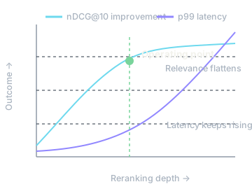
Then repeat the experiment for reranking depth.

10 candidates
25 candidates
50 candidates
100 candidates
200 candidates

Measure:

nDCG@10 improvement
vs
added p99 latency

Eventually the relevance curve flattens while the latency curve keeps climbing.

That is where production engineering begins.

---

26. Choosing a Stack

For a learning project, an integrated Lucene-based engine is hard to beat because it exposes many real production concerns in one system:

BM25
segments
merges
shards
query-then-fetch
HNSW
hybrid retrieval
caching
thread pools
backpressure

OpenSearch remains Apache-2.0 licensed.

Elasticsearch has a different licensing model: free portions of the source can be used under AGPLv3, SSPL, or ELv2, while Elastic’s default distribution remains under ELv2.

A dedicated vector database is useful when vector retrieval is the central workload, especially where filtering, vector lifecycle management, or specialized ANN capabilities are important.

For learning, though, I would optimize less for choosing the fashionable database and more for exposing the tradeoffs you want to understand.

A boring architecture with good measurements teaches more than an impressive architecture with none.

---

27. The Main Production Lessons

The most important thing I learned while digging into production search is that the retrieval algorithm is only one layer of the problem.

An inverted index explains how lexical retrieval works.

BM25 explains why some matching documents score above others.

HNSW explains how semantic retrieval becomes fast enough to serve.

But production search starts when those components interact with:

index freshness
sharding
fan-out
tail latency
memory pressure
caches
reranking
backpressure
reindexing
observability

The architecture is therefore less:

query -> algorithm -> answer

and more:

query
  -> generate candidates
  -> spend increasingly more computation
  -> stop spending computation when it stops being useful
  -> survive distributed-system variance
  -> return something before the user notices

That final constraint changes almost every design decision.

A search engine with perfect relevance and three-second p99 latency is usually a bad search engine.

A search engine with 10ms latency that never retrieves the relevant document is also a bad search engine.

Production search lives in the space between those two failures.

And most of the engineering work is deciding exactly where in that space your product should operate.